Table of Contents
This page describes benchmark results of different implementations and algorithms of CRFs.
This is the list of CRF implementations and versions (the latest as of 1st July 2011) used for the experiments.
The experiments use the training and test sets of CoNLL 2000 chunking shared task. We employ the same feature set among different CRF implementations; state (unigram) and transition (bigram) features are generated from the training and test sets by applying the feature template bundled in CRF++. For CRFsuite and MALLET, the state observations (attributes) that are compatible to the feature template are generated by a script program (refer to the tutorial for more information). The training data contains 8936 sentences (sequences), 338,574 attributes, and 22 labels. The test data contains 2012 sentences.
In this experiment, the following parameters were specified for the implementations:
- L2 regularization (C = 1.0, rho = 0.70710678118654746)
- Stopping criterion for L-BFGS: delta = 1e-5, period = 10
- Maximum number of iterations for averaged perceptron is 50
All of the experiments were run on Ubuntu 10.10 (AMD64) (with gcc 4.4.5), Six-Core Opteron 2435(2.6GHz) x 2 processors, 64GB main memory.
In general, it is difficult to compare different implementations in terms of training speed since the implementations may produce different numbers of features, use different algorithms for updating feature weights, and finish training processes in different criteria (e.g., convergence criterion of L-BFGS/SGD). In addition, we need to check whether CRF models obtained from different implementations show the similar accuracy on the test data.
Figure 1 shows seconds elapsed for one L-BFGS/SGD iteration, where each implementation processes all instances in the training data once and update feature weights. Although it depends on implementations what has done in one iteration (e.g., computing forward-backward scores, observation/model expectations of features, Viterbi probabilities, and updates of feature weights), these figures characterize speed optimizations of implementations. The training speed is also affected by the number of features (or strategy of feature generation) used in training. The numbers of features for sparse and dense models are 450,000-600,000 and ca. 7,500,000, respectively.
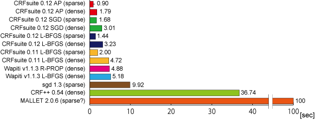
In summary, CRFsuite (L-BFGS; dense) is 1.6 times faster than Wapiti (L-BFGS), 3.1 times faster than sgd, 11.4 times faster than CRF++, 31.0 times faster than MALLET on training. CRFsuite 0.12 is about 1.5 times faster than the older version (0.11). L-BFGS and SGD implemented in CRFsuite are roughly comparable in terms of the computational costs for updating feature weights in one iteration. However, this does not mean that L-BFGS and SGD are equally fast; as we will see, SGD improves the log-likelihood of the model more drastically than L-BFGS does in one iteration. In other words, SGD approaches to the optimal weights in less iterations than L-BFGS.
Focussing more on the comparison of L-BFGS and SGD in CRFsuite, we notice that L-BFGS is slightly faster than SGD with less features while L-BFGS is slower with more features. This is because the computational costs of L-BFGS and SGD are O(adn + bk) and O(cdn), respectively. Here:
- d is the average number of features that are relevant to an instance
- n is the number of instances
- k is the number of features
- a is the constant factor for computing gradients of an instance
- b is the constant factor in which L-BFGS updates feature weights in one iteration
- c is the constant factor in which SGD updates feature weights for an instance
Usually, a < c; thus, L-BFGS may run faster than SGD while the number of features (k) is small.
Table 1 reports the full result of the experiment. All implementations roughly achieve the similar performance in terms of accuracy. SGD implementations stop after 100 iterations since sgd 1.3 has no functionality to test the convergence of log-likelihood. In general, SGD appears to be more efficient than L-BFGS.
Table 1. Performance of training
| Software | Solver | Feature | # Features | Time | # Iters | Update | Loss | Acc | Log |
|---|---|---|---|---|---|---|---|---|---|
| [s] | [s/ev] | [%] | |||||||
| CRFsuite 0.12 | AP | sparse | 452 755 | 48.1 | 50 | 0.9 | 5.5 | 95.760 | Log |
| CRFsuite 0.12 | AP | dense | 7 385 312 | 93.7 | 50 | 1.8 | 3.4 | 95.930 | Log |
| CRFsuite 0.12 | L2-SGD | sparse | 452 755 | 589.4 | 345 | 1.7 | 13 181.6 | 96.000 | Log |
| CRFsuite 0.12 | L2-SGD | dense | 7 385 312 | 1 052.1 | 345 | 3.0 | 11 635.9 | 96.010 | Log |
| CRFsuite 0.12 | L-BFGS | sparse | 452 755 | 262.3 | 165 | 1.4 | 13 139.4 | 95.990 | Log |
| CRFsuite 0.12 | L-BFGS | dense | 7 385 312 | 636.8 | 159 | 3.2 | 11 602.6 | 96.010 | Log |
| CRFsuite 0.11 | L-BFGS | dense | 452 799 | 330.3 | 140 | 2.0 | 13 125.2 | 95.980 | Log |
| CRFsuite 0.11 | L-BFGS | sparse | 7 385 356 | 796.2 | 132 | 4.7 | 11 596.8 | 96.020 | Log |
| Wapiti v1.1.3 | R-PROP | dense | 7 448 122 | 165.2 | 33 | 4.9 | 33 937.2 | 95.817 | Log |
| Wapiti v1.1.3 | L-BFGS | dense | 7 448 122 | 1 292.5 | 226 | 5.2 | 24 872.9 | 95.753 | Log |
| sgd 1.3 | L2-SGD | sparse | 338 552 | 1 012.7 | 100 | 9.9 | 3 143.2 | 96.038 | Log |
| CRF++ 0.54 | MIRA | dense | 7 448 606 | 14 114.0 | 175 | ? | 770.7 | 95.724 | Log |
| CRF++ 0.54 | L-BFGS | dense | 7 448 606 | 4 985.8 | 131 | 36.7 | 7 713.5 | 96.070 | Log |
| MALLET 2.0.6 | L-BFGS | sparse? | 592 965 | 11 858.8 | 105 | 100 | 7 682.2 | 95.762 | Log |
- # Features
- Number of features generated by a training program. These numbers vary depending especially on the treatment of negative features. For example, CRF++ generates all of possible features, whereas crfsgd does positive features only. In this experiment, we call the former strategy for feature generation as dense and the latter as sparse. CRFsuite can use the both strategies by configuring options for training. Since the speed and memory space for training are greatly affected by the number of features, we need to compare implementations within each group, i.e., CRFsuite (sparse) vs crfsgd vs MALLET and CRFsuite (dense) vs Wapiti vs CRF++.
- Time [s]
- The total time, in seconds, elapsed while a training process alives. In general, shorter is better.
- # Iters
- The number of iterations that an implementation used for training. The definition of 'iteration' of CRFsuite (L-BFGS) is different from the one of CRF++. CRFsuite does not count objective-function evaluations invoked by the line-search trials as iterations, whereas CRF++ include ones.
- Update [s/ev]
- The averaged elapsed time, in seconds, for an iteration. These figures are identical to ones shown in Figure 1. We can use these figures as an indicator for the 'goodness' of the implementations.
- Loss
- The final value of the loss (negative of regularized log-likelihood) of each implementation. In general, a smaller value indicates that the model fits to the training data better. However, the definition of a loss in one implementation may be different from that for another implementation. Therefore, we cannot compare these values directly to assess the 'goodness' of training algorithms.
- Acc [%]
- Item accuracy of a CRF model on the test data. These figures are only for validating the correctness of this experiment; we can say that this experiment is fair since CRF models with each feature set (sparse or dense) performed roughly at the same accuracy.
In the section called “Training speed”, we showed that L-BFGS and SGD are comparable in terms of the computational cost for updating feature weights in one iteration. However, this does not mean that these algorithms approach to the optimal model at the same speed.
Figure 2 plots objective values at each iteration. Each training algorithm tries to minimize the objective value to fit the model to the training data. The definitions of objective values vary depending on training algorithms: negative of L2-regularized log-likelihood for L-BFGS and SGD, and average number of mislabeled items per instance for Averaged Perceptron. Even though we cannot compare L-BFGS and SGD with Averaged Perceptron (AP), the difference of L-BFGS and SGD is obvious from this figure; L-BFGS approaches to the solution more slowly (at iterations 1 to 40) than SGD.
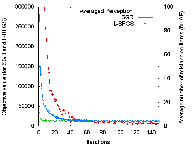
Figure 3 shows accuracy values measured on the test data at each iteration of the training data. SGD and Averated Perceptron achieved as high as 95.13% and 95.27% accuracy, respectively, after the first iteration whereas L-BFGS obtained only 62.71%. L-BFGS required 22 iterations to reach the level of 95% accuracy. In the end, L-BFGS and SGD show the similar accuracy (about 96%). In contrast, Averaged Perceptron achieved 95.9% accuracy at iteration 8, and gradually dropped its performance. It may be important to tune the parameter of number of iterations for Averaged Perceptron.
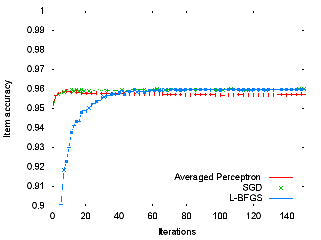
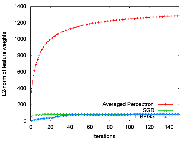
Figure 4 presents the L2-norm of feature weights at each iteration.